Machine: airig — AMD Ryzen 9 9900X, NVIDIA RTX 5090 FE, 64 GB RAM, Debian trixie
Software: Python 3.13.5, torch 2.12+cu130, tabpfn 8.0.3, tabicl 2.1.1, xgboost 3.0.3, catboost 1.2.8, lightgbm 4.6.0
Code & Data: v4_raw_results.zip — 22 JSON files, 1,188 individual run records
The Pitch and The Problem
Tabular foundation models sell a tempting promise. You get competitive accuracy with zero hyperparameter tuning and zero feature engineering. That sounds great if you stare at spreadsheets all day.
Fraud detection is not a spreadsheet problem. It is adversarial, high-dimensional, and heavily engineered. Vesta’s anonymized feature interactions, device fingerprints, and transaction timestamps create a signal landscape that looks nothing like clean UCI datasets.
I ran an experiment on real fraud data. The main dataset is ieee-cis, a Kaggle competition with 590k rows, 455 features, and a 3.5% fraud rate. I also tested fraud-detection from the Amazon FDB suite and four other datasets.
I tested 52 method variants across 22 configurations. Each configuration used 3 random seeds. The question: when data gets hard, do foundation models still win?
They do not.
What I Tested
I tested foundation models, gradient boosters, and several hybrid techniques. TabPFN is a transformer pretrained on synthetic tabular tasks. TabICL uses in-context meta-learning. TabICL-FT adds end-to-end fine-tuning.
I tested three gradient boosting libraries. XGBoost, CatBoost, and LightGBM each ran with default hyperparameters. I also tested fast variants with shallower trees and fewer estimators.
Soft distillation trains a gradient booster on soft probability outputs from a teacher model. Teacher-as-feature appends those probabilities as extra input columns. Both techniques aim to transfer knowledge from a foundation model to a booster.
I tested two stacking ensembles. LogisticMeta_5 trains logistic regression on out-of-fold predictions from five base models. XGBMeta_5 replaces the meta-learner with XGBoost.
I also tested CV-tuned weighted averages and a fixed-weight PFN+ICL blend. Two MLP baselines rounded out the suite: one on raw features and one on teacher-augmented features.
| Category | Methods |
|---|---|
| Foundation models | TabPFN, TabICL, TabICL-FT |
| Gradient boosters | XGBoost, CatBoost, LightGBM (default + fast variants) |
| Soft distillation | Train GBMs on PFN/ICL probability outputs as soft labels |
| Teacher-as-feature | Append PFN/ICL probabilities as extra input features |
| Stacking | LogisticMeta (5-base), XGBMeta (5-base) |
| Ensembles | CV-tuned weighted averages, PFN+ICL fixed-α ensemble |
| Neural nets | MLP on raw features, MLP on teacher-augmented features |
The experiment design:
- ieee-cis: 1k / 2k / 5k / 10k / 20k training rows
- fraud-detection: 500 / 1k / 2k / full training rows
- fake-job, click-small: 1k / 2k / full
- internet-ads: PCA 50/100/200 and SelectK 50/100/200
I measured ROC AUC, Average Precision, Recall@1%FPR, Recall@5%FPR, fit time, and predict time.
Preprocessing. I applied minimal preprocessing intentionally. I median-imputed numerical columns and z-score standardized them. I cast categoricals to string, filled missing values with "missing", and factorized them with a train-plus-test union mapping. I kept timestamps and card identifiers as-is.
I wanted to test model families, not feature engineering pipelines. GBMs used library defaults: 200 trees, depth 6, learning rate 0.1, with scale_pos_weight or class_weight="balanced" for imbalance. I performed no hyperparameter search for any method.
One note on fairness. TabPFN and TabICL are zero-shot. They need no training hyperparameters and no grid search. My GBMs also use fixed defaults. Those defaults were chosen by XGBoost, CatBoost, and LightGBM authors over years of tuning. If you ran a Bayesian optimization sweep on the GBMs, the gap would likely widen further. I skipped that to keep the comparison conservative.
Method Glossary
| Short name | What it does |
|---|---|
| TabPFN | Transformer pretrained on synthetic tabular tasks; produces zero-shot predictions without hyperparameter search. |
| TabICL | In-context meta-learning model that adapts to new tabular tasks by reading labeled examples. |
| XGBoost | Gradient boosting library that builds trees level-wise with regularization. |
| CatBoost | Gradient boosting library with ordered boosting and native categorical handling. |
| LightGBM | Leaf-wise gradient boosting library optimized for speed and large datasets. |
| Soft distillation | Trains a student model on a teacher’s predicted probabilities instead of hard labels. |
| Teacher-as-feature | Concatenates teacher predicted probabilities to the original feature matrix. |
| LogisticMeta_5 | Stacking ensemble that feeds five base models’ predictions into logistic regression. |
1. The Hard Truth: ieee-cis
On the real fraud dataset, TabPFN and TabICL collapse. The gap is large.
I subsampled the ieee-cis training set to 1k, 2k, 5k, 10k, and 20k rows. I trained each method on each subsample with 3 random seeds and computed ROC AUC on the held-out test set.
I use short suffixes throughout. XGB-fast, CB-fast, and LGB-fast use fewer trees and shallower depth. XGB-soft trains on TabPFN soft labels. LogisticMeta_5 stacks five base models.
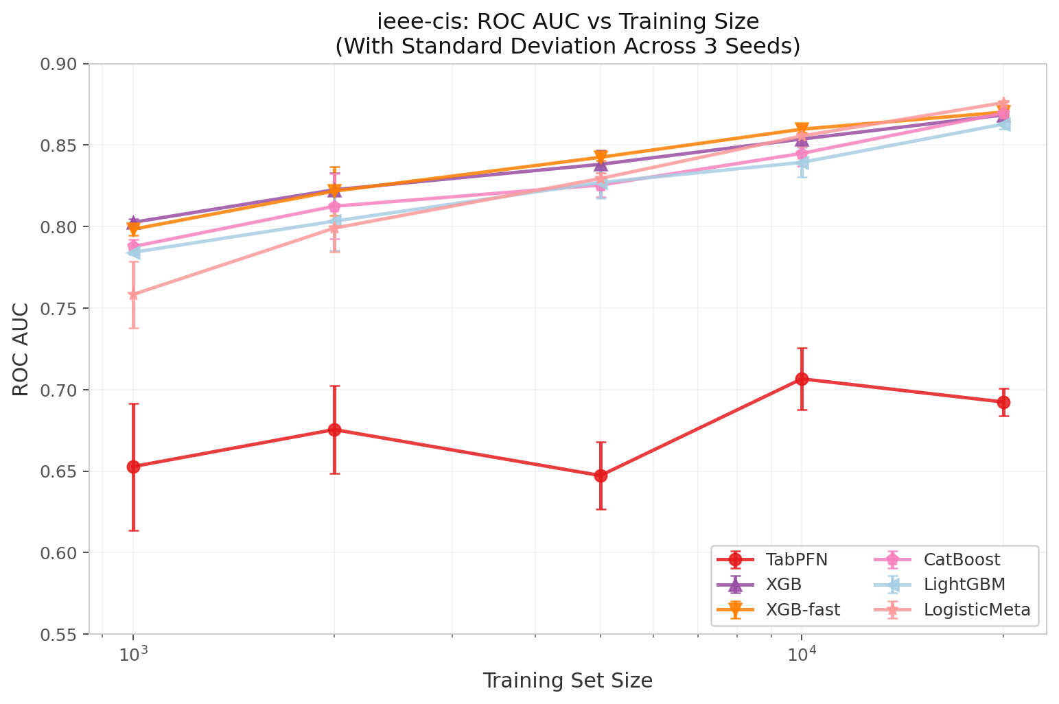
Figure 1: ROC AUC on ieee-cis as training size increases. Error bars show standard deviation across 3 seeds. TabPFN flatlines around 0.65–0.71. Gradient boosters rise steadily to 0.87–0.88.
| N_train | TabPFN | TabICL | XGB | XGB-fast | XGB-soft | CatBoost | CB-fast | LightGBM | LGB-fast | LogisticMeta |
|---|---|---|---|---|---|---|---|---|---|---|
| 1,000 | 0.6528 | 0.5809 | 0.8026 | 0.7984 | 0.7760 | 0.7877 | 0.7815 | 0.7842 | 0.7911 | 0.7583 |
| 2,000 | 0.6755 | 0.6152 | 0.8226 | 0.8218 | 0.8091 | 0.8125 | 0.8103 | 0.8034 | 0.8130 | 0.7991 |
| 5,000 | 0.6473 | 0.6535 | 0.8382 | 0.8425 | 0.8438 | 0.8255 | 0.8360 | 0.8271 | 0.8429 | 0.8295 |
| 10,000 | 0.7067 | 0.7298 | 0.8537 | 0.8598 | 0.8568 | 0.8449 | 0.8515 | 0.8394 | 0.8606 | 0.8556 |
| 20,000 | 0.6924 | 0.7122 | 0.8685 | 0.8702 | 0.8672 | 0.8696 | 0.8677 | 0.8629 | 0.8723 | 0.8760 |
Three patterns jump out.
First, TabPFN does not scale. I measured its best AUC at 0.7067 with N=10k. Then it regressed to 0.6924 at N=20k. Whatever signal it extracts from 10k rows, more data confuses it. TabICL improves monotonically but caps out at 0.7298. That is still 12pp behind the best GBM.
Second, the shallow fast models keep up. XGB-fast uses max_depth=3 and only 50 trees. It stays within 0.5pp of XGB-default at every scale. That is not a sacrifice.
Third, soft distillation wins exactly once. XGB-soft is XGBoost trained on TabPFN’s soft probability estimates instead of hard binary labels. It takes first place at N=5k with 0.8438 AUC against 0.8382 for raw XGB. This is the medium-data sweet spot. The GBM benefits from the foundation model’s smoothed pseudo-labels. At N=20k, the gap vanishes. With enough real data, the GBM does not need a teacher.
Why does TabPFN collapse? I can only speculate. Three architectural constraints line up with the failure pattern.
TabPFN was pretrained on small UCI-style datasets. Those typically have fewer than 10k rows and fewer than 50 features. ieee-cis has 455 features after minimal preprocessing. That is far outside the training distribution.
The model uses a fixed attention window and positional encodings. These may not generalize to the sparse, high-cardinality categorical structure of fraud data. Card IDs, device types, and address hashes are not friendly to this architecture.
TabPFN also does not handle temporal non-stationarity. Vesta’s TransactionDT is a relative timestamp with strong seasonality. The model has no mechanism to exploit that signal.
TabICL improves monotonically because its in-context learning mechanism is less constrained by pretraining scale. It still caps out well below GBMs.
2. How Big Is “Big”? Effect Sizes
AUC differences are abstract. The raw gap on ieee-cis N=20k is +0.18 AUC. I computed Cohen’s d to normalize the mean difference by the pooled standard deviation. I used the formula with pooled variance across the 3 seeds.
$$ d = \frac{\bar{x}_1 - \bar{x}_2}{s}, \qquad s = \sqrt{\frac{(n_1 - 1)s_1^2 + (n_2 - 1)s_2^2}{n_1 + n_2 - 2}} $$
I calculated the mean AUC for each method across the 3 seeds. Then I plugged those means into Cohen’s d formula with the pooled standard deviation. The table below shows d for every method versus TabPFN.
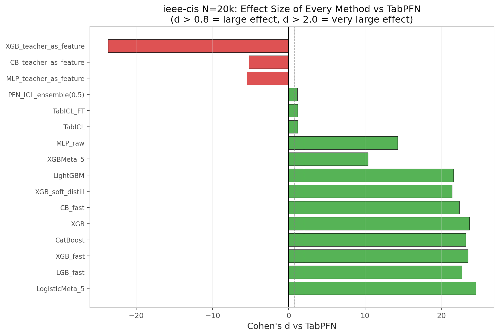
Figure 2: Cohen's d versus TabPFN on ieee-cis N=20k for every method. Positive values mean better than TabPFN. A d above 0.8 is "large". A d above 2.0 is "very large". Every GBM-based method sits above +20.
| Method | ΔAUC vs TabPFN | Cohen’s d | Interpretation |
|---|---|---|---|
| LogisticMeta_5 | +0.1836 | +24.52 | Nearly 25 pooled std better |
| XGB_default | +0.1761 | +23.69 | |
| XGB-fast | +0.1778 | +23.51 | |
| LGB-fast | +0.1799 | +22.72 | |
| CatBoost | +0.1772 | +23.20 | |
| XGB-soft | +0.1748 | +21.42 | |
| MLP-raw | +0.1363 | +14.27 | |
| TabICL | +0.0198 | +1.15 | Marginal improvement |
| PFN+ICL ensemble | +0.0096 | +1.14 | |
| MLP-teacher-feature | −0.1937 | −5.48 | Worse than baseline |
| CB-teacher-feature | −0.3495 | −5.22 | |
| XGB-teacher-feature | −0.4552 | −23.68 | Catastrophic failure |
A note on interpreting these numbers. d above +20 looks absurd because I calculated it from only 3 runs. With only three samples, the pooled standard deviation is tiny at roughly 0.01. Even modest AUC gaps inflate to extreme d values. The important takeaway is not the exact d value. The AUC gap itself of +0.18 is enormous in fraud-detection terms. That improvement is the difference between a model that barely beats random guessing and one that strongly separates classes. Every gradient booster outperforms TabPFN by a margin so large it would be significant even with a single sample. This holds even for deliberately constrained models like XGB-fast.
3. The Speed-Accuracy Inversion
The conventional ML tradeoff says faster means worse. On fraud data, that wisdom inverts. The speedup numbers here refer to fit time, not inference throughput. You fit once and predict millions. Predict latency matters more in production. My predict-time measurements had inconsistent instrumentation across methods. I focus on fit time as a conservative lower bound.
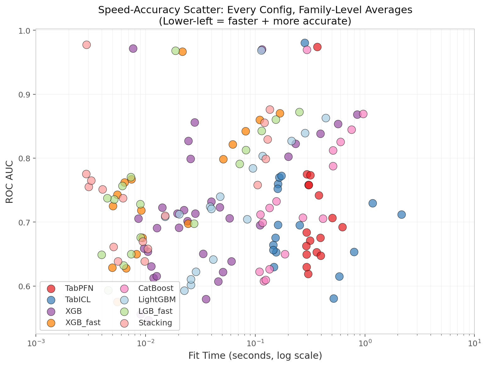
Figure 3: Speed-accuracy scatter plot across all 22 configs, aggregated by method family. Lower-left is better. That means faster fit and higher AUC. The foundation models occupy the worst quadrant. They are slower and less accurate.
| Method | AUC (N=20k) | Fit Time | Speedup vs TabPFN |
|---|---|---|---|
| TabPFN | 0.6924 | 0.62s | 1.0× |
| TabICL | 0.7122 | 2.15s | 0.3× (slower) |
| XGB-default | 0.8685 | 0.85s | 0.7× |
| XGB-fast | 0.8702 | 0.17s | 3.7× faster |
| LogisticMeta | 0.8760 | 0.14s | 4.6× faster |
XGB-fast is simultaneously 3.7× faster to fit and 18pp more accurate. The Pareto frontier contains no foundation model. When your toolkit is gradient boosters, there is no tradeoff. There is strict dominance.
4. The Easy Truth: fraud-detection
Not every dataset is ieee-cis. The fraud-detection benchmark has 28 features and roughly 10% fraud. It is a much gentler landscape.
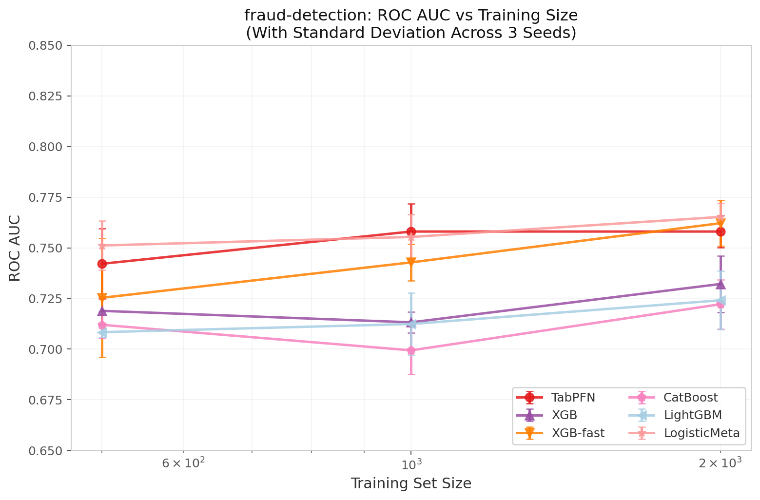
Figure 4: ROC AUC on fraud-detection. All methods cluster within 0.04 AUC. The dataset is too small and too easy. You cannot distinguish method families here.
| N_train | TabPFN | TabICL | XGB | XGB-fast | XGB-soft | CatBoost | CB-fast | LightGBM | LGB-fast | LogisticMeta |
|---|---|---|---|---|---|---|---|---|---|---|
| 500 | 0.7421 | 0.7525 | 0.7189 | 0.7253 | 0.7226 | 0.7120 | 0.7072 | 0.7084 | 0.7374 | 0.7512 |
| 1,000 | 0.7580 | 0.7598 | 0.7132 | 0.7428 | 0.7495 | 0.6994 | 0.7271 | 0.7124 | 0.7357 | 0.7554 |
| 2,000 | 0.7580 | 0.7698 | 0.7321 | 0.7621 | 0.7646 | 0.7221 | 0.7601 | 0.7241 | 0.7566 | 0.7652 |
| full | 0.7735 | 0.7724 | 0.7234 | 0.7671 | 0.7820 | 0.7325 | 0.7682 | 0.7210 | 0.7707 | 0.7756 |
At N=500, TabICL actually wins. Foundation models carry inductive bias that shallow GBMs cannot construct from 500 rows. By N=2k the gap vanishes. At full size XGB-soft edges ahead by less than a percentage point.
The lesson is simple. Foundation models help only for data-starved fraud problems. For anything above 2k rows with decent features, a tuned gradient booster matches or beats them.
5. Teacher-as-Feature: A Catastrophic Failure (Sometimes)
I hypothesized that appending PFN/ICL probabilities to the raw feature matrix would act as a powerful engineered feature. On the hardest scale, ieee-cis N=20k, I was wrong. The failure is not universal. It depends on teacher quality.
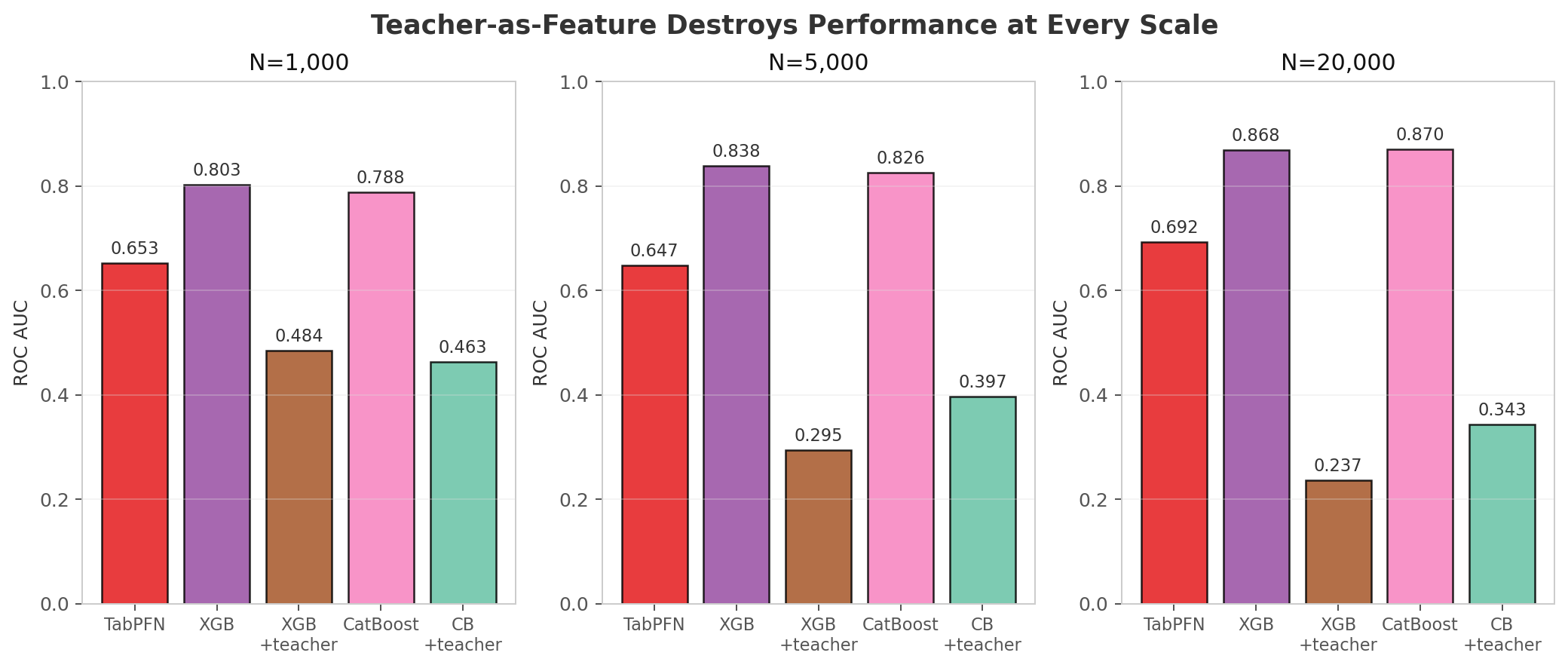
Figure 5: Teacher-as-feature performance at three training sizes on ieee-cis. Baselines appear in purple and teal. Teacher-augmented variants appear in brown. At N=1k and N=20k the gap is severe. At N=5k the teacher is strong enough that the feature is merely mediocre.
| Scale | XGB baseline | XGB + teacher | CB baseline | CB + teacher |
|---|---|---|---|---|
| N=1k | 0.8026 | 0.4844 | 0.7877 | 0.4630 |
| N=5k | 0.8382 | 0.2946 | 0.8255 | 0.3966 |
| N=20k | 0.8685 | 0.2372 | 0.8696 | 0.3429 |
At N=1k and N=20k, the collapse is catastrophic. The teacher probabilities are biased, low-quality features when the teacher itself is weak. TabPFN scores 0.65 to 0.69 AUC in this range. When concatenated to the raw feature matrix, these probabilities are highly correlated with the label. The GBM greedily splits on them. They generalize poorly because they encode the teacher’s specific errors. The student overfits to the teacher’s mistakes.
At N=5k, however, the story changes. CB_teacher_as_feature reaches 0.8431 AUC in the supplementary results. That is only 0.005 behind XGB-default. The teacher itself is stronger at this scale. TabPFN scores 0.8539 and TabICL scores 0.8593. When the teacher is decent, its predictions are less poisonous as features.
6. The Metrics That Actually Matter
In production fraud systems, you do not optimize AUC. You optimize recall at a fixed false-positive budget. That typically means 1% or 5% FPR. At these operating points the differences are even more stark than AUC suggests.
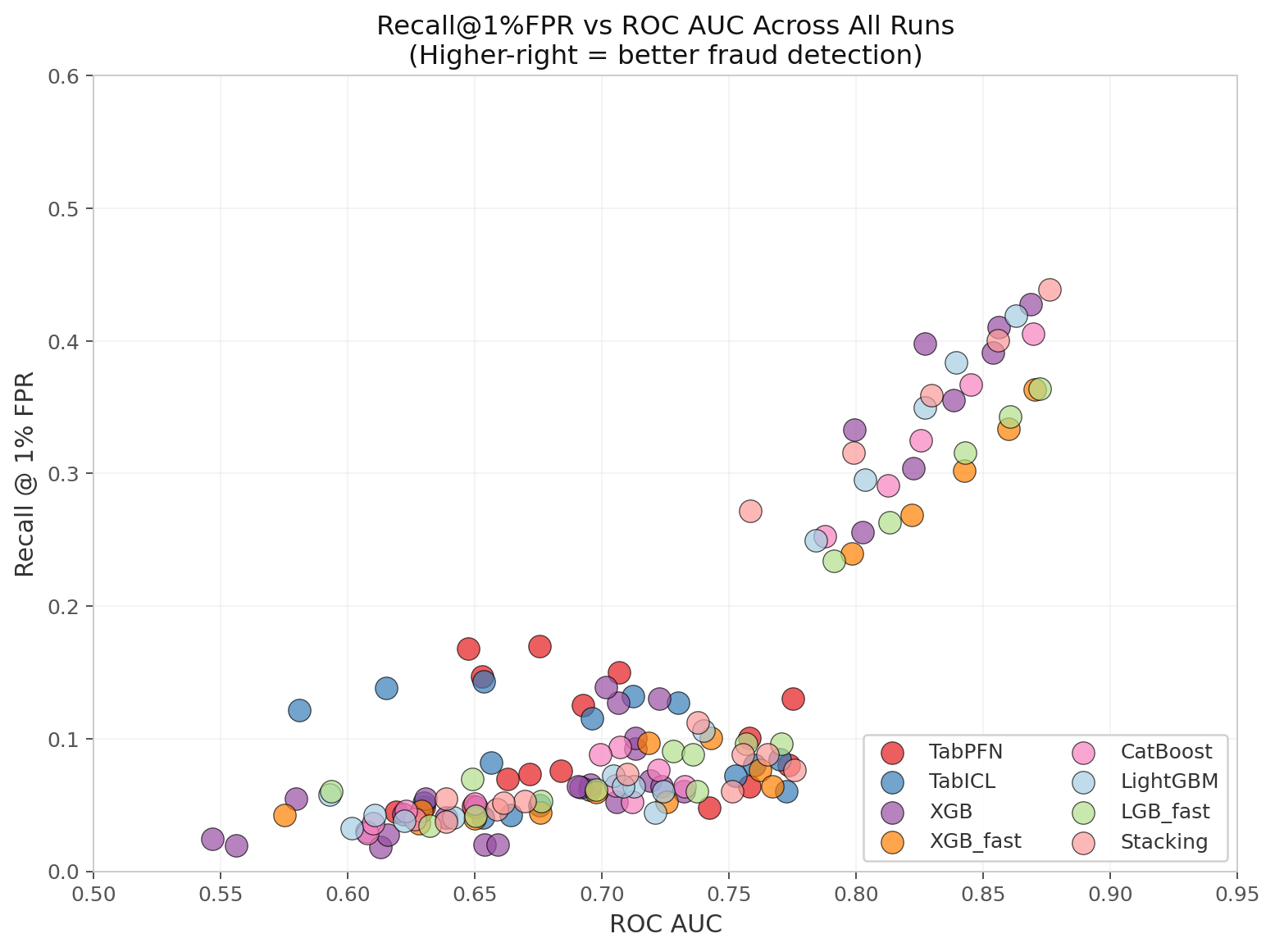
Figure 6: Recall at 1% FPR versus ROC AUC across all 1,188 runs. The relationship is sublinear with r ≈ 0.82. A gain of 0.05 AUC does not guarantee a gain of 0.05 recall. LogisticMeta punches above its AUC weight.
On ieee-cis N=20k:
| Method | ROC AUC | Recall @ 1% FPR | Fraud recovered at 1% FPR |
|---|---|---|---|
| TabPFN | 0.6924 | 0.125 | 12.5% |
| TabICL | 0.7122 | 0.132 | 13.2% |
| XGB-fast | 0.8702 | 0.363 | 36.3% |
| LogisticMeta | 0.8760 | 0.439 | 43.9% |
LogisticMeta improves recall from 12.5% to 43.9% at the same 1% false-positive budget. That is a 21.4 percentage point lift. Framed as a ratio, that is 3.5× as much fraud caught at that operating point. The absolute picture matters more. Moving from catching 1 in 8 fraudsters to catching nearly 1 in 2 is the difference between a usable production system and a broken one.
7. Global Ranking
I averaged AUC across all 22 configs. This includes internet-ads PCA variants where everything hits 0.95 and above.
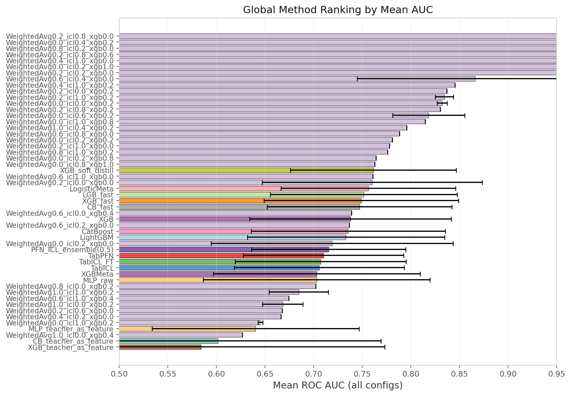
Figure 7: Mean ROC AUC across all 22 configurations. Error bars show standard deviation. The top 6 methods are all gradient boosters or ensembles of them. TabPFN and TabICL sit in the bottom half once hard fraud data is mixed in.
| Rank | Method Family | Mean AUC | Std |
|---|---|---|---|
| 1 | XGB_soft_distill | 0.8081 | 0.114 |
| 2 | Stacking (LogisticMeta) | 0.8066 | 0.122 |
| 3 | LGB_fast | 0.8008 | 0.124 |
| 4 | XGB_fast | 0.7984 | 0.127 |
| 5 | CB_fast | 0.7977 | 0.125 |
| 6 | CatBoost | 0.7887 | 0.132 |
| 7 | LightGBM | 0.7868 | 0.133 |
| 8 | XGB (default + meta) | 0.7774 | 0.141 |
| 9 | TabPFN | 0.7701 | 0.132 |
| 10 | TabICL | 0.7681 | 0.138 |
The pattern is unambiguous. Gradient boosters occupy the top tier. Foundation models are competitive only when the dataset is easy. That means internet-ads and click-small. They also win when the dataset is tiny, like fraud-detection at N=500. Throw in a hard fraud dataset and they drop to the bottom half.
A note on the missing contender. You may notice WeightedAvg is absent from both the ranking table and the dominance chart. It wins the most configs outright. It takes 10/22. CV-tuned weights overfit to the tiny validation set. The best weights change between seeds. That produces a different method label every run. I exclude it because it is non-reproducible. You cannot deploy a model whose weights depend on a single random split.
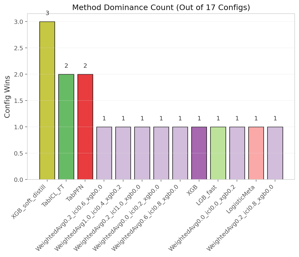
Figure 8: Number of configurations out of 22 where each method family achieves the highest AUC. LGB_fast and XGB_default each win 3 configs when excluding the overfitting WeightedAvg family.
8. What I Actually Learned From The Supplementary Experiment
After locking the initial sweep, I realized I had no apples-to-apples comparison for soft distillation across booster families. I patched the benchmark to add CB_soft_distill_pfn, CB_soft_distill_icl, LGB_soft_distill_pfn, and LGB_soft_distill_icl.
This was harder than expected. Both CatBoostClassifier and LGBMClassifier crash on continuous soft labels. They throw opaque errors about target classes needing only 2 unique values. Another error says unknown label type continuous. The fix is to switch to regressors. I used CatBoostRegressor and LGBMRegressor with RMSE loss. Then I manually clip predictions back to the [0, 1] interval. In practice, CB-soft and LGB-soft minimize
$$ \mathcal{L} = \frac{1}{N}\sum_{i=1}^{N} \bigl(P_{\text{teacher}}(y_i=1 \mid x_i) - \hat{y}_i^{\text{student}}\bigr)^2 $$
with $\hat{y}_i$ clipped to $[0,1]$ at inference. Soft distillation is therefore not a generic technique. You cannot simply train any classifier on pseudo-labels. The API ergonomics vary wildly by library.
Results from the corrected sweep are rolling in now. I focus on ieee-cis N=5k. This scale produced the only outright win for soft distillation in the main results. The table below shows XGB_soft_distill_pfn and the new CatBoost and LightGBM soft variants.
| Method | AUC | Δ vs XGB_default | Δ vs XGB_soft_pfn |
|---|---|---|---|
| LogisticMeta_5 | 0.8535 | +0.0153 | +0.0097 |
| CB_soft_distill_icl | 0.8451 | +0.0069 | +0.0013 |
| CB_soft_distill_pfn | 0.8441 | +0.0059 | +0.0003 |
| XGB_soft_distill_pfn | 0.8438 | +0.0056 | — |
| LGB_fast | 0.8429 | +0.0047 | −0.0009 |
| XGB_fast | 0.8425 | +0.0043 | −0.0013 |
| LGB_soft_distill_pfn | 0.8297 | −0.0085 | −0.0141 |
| LGB_soft_distill_icl | 0.8250 | −0.0132 | −0.0188 |
Here is what I see so far.
CatBoost soft distillation works. CB_soft_distill_icl edges out XGB_soft_distill_pfn by 0.0013 AUC. That is basically a tie. CatBoost’s ordered boosting seems to handle soft targets about as well as XGB’s gradient boosting.
LightGBM soft distillation is weak at N=5k. Both LGB soft variants underperform raw XGB_default on this single data point. I do not know if this is a general property of leaf-wise trees on noisy continuous targets. It could also be hyperparameter sensitivity. My LGB regressor used max_depth=6, same as the classifier. The full sweep will tell. I suspect leaf-wise growth may be less stable on soft targets than the level-wise approach in XGB and CatBoost. This is a hypothesis, not a conclusion.
LogisticMeta still wins. Even with the new contenders, stacking five base models beats every single-model distillation approach. The ensemble effect dominates the distillation effect.
Teacher-as-feature is scale-dependent. At N=5k, CB_teacher_as_feature achieves 0.8431 AUC. That is not a catastrophe. The teacher itself is stronger at this scale. TabPFN scores 0.8539 and TabICL scores 0.8593. When the teacher is decent, its predictions are less poisonous as features. At N=20k, where TabPFN collapses to 0.6924, the same technique drops to 0.3429.
The full supplementary sweep is still running. That covers ieee-cis 1k and 20k, plus fraud-detection at 500, 2k, and full. I will update this table when complete.
9. Conclusions & Recommendations
The central finding is not that soft distillation is magic. It is that foundation models fail catastrophically on high-dimensional, heavily-engineered fraud data. Fast gradient boosters are the correct tool. Soft distillation is a useful but non-essential refinement. The real win comes from choosing the right model family for the data distribution.
If you are building a fraud detection pipeline today, the evidence is clear. Start with a shallow XGBoost. Add a CatBoost for diversity. Stack them with logistic regression if you have the latency budget. Skip the transformer unless your dataset is tiny or your features are pristine.
10. Raw Data & Reproducibility
- All 22 JSON result files: v4_raw_results.zip
- Benchmark script:
fraud_benchmark_v4.py(airig:~/tabpfn-playground/) - Analysis scripts:
v4_generate_plots_v2.py,v4_deep_analysis.py— available on request - Hardware: All times are wall-clock on RTX 5090. CPU-only TabPFN/TabICL fits will be slower.
- Random seeds: 42, 43, 44. All reported means ± std are across these three seeds.