I ran the entire shootout on a single workstation named airig — AMD Ryzen 9 9900X, NVIDIA RTX 5090 FE, 64 GB RAM. If you want to reproduce these numbers, start with that hardware baseline.
The software stack is locked to Python 3.13.5, torch 2.12+cu130, tabpfn 8.0.3, tabicl 2.1.1, xgboost 3.2.0, catboost 1.2.7, and lightgbm 4.6.0. I pinned every version because one point release can reshuffle the entire feature-importance leaderboard.
All raw results are dumped into ten JSON files: fi_credit_g.json, fi_telco_churn.json, fi_bank_marketing.json, fi_Credit_Card_Fraud_Classification.json, fi_default_of_credit_card_clients.json, distill_creditg.json, distill_telco.json, distill_bank.json, distill_cc_fraud.json, and distill_default.json.
You can regenerate all of them with feature_importance_cmp.py and distill_engineered.py, assuming your environment matches the spec above. If you rerun this on a 4090 or a newer PyTorch nightly, I want to know which rankings survive.
The puzzle
TabPFN3 and TabICL are Bayesian prior-based foundation models for tabular classification. XGBoost is a gradient-boosted decision tree.
They share almost no architectural DNA: one uses cross-attention over in-context learning examples, the other uses axis-parallel splits on single features. You would naturally expect them to extract completely different signal from the same data.
I stacked them with a logistic meta-learner on five classification datasets. On four of them, the ensemble was underwhelming—it matched or barely beat the best standalone model, adding only +0.1 to +0.5 pp.
Hardly worth the complexity.
Then I tested cc-fraud, a credit-card fraud dataset with a 0.17% positive rate. The ensemble was dramatically more robust.
TabPFN3 alone dropped to 96.99% AUC on one run, but the meta-learner never fell below 98.34%.
I’m now hunting for the boundary condition: is extreme class imbalance the only scenario where attention-based and tree-based models produce complementary enough errors to justify a meta-learner?
Hypothesis
I’ve watched too many ensemble pipelines eat GPU hours just to deliver the same accuracy as a single model. It’s the kind of result that makes you question why you bothered with stacking at all.
The real problem isn’t the meta-learner. It’s whether your base models are actually seeing different things. When XGBoost and TabPFN attend to different features, their errors become uncorrelated. One stumbles where the other succeeds, so the meta-learner has genuine diversity to work with.
When they lock onto the same features, the opposite happens. Their errors correlate perfectly, and the meta-learner simply averages two copies of the identical mistake.
This suggests a cheap diagnostic: measure how much their feature importances disagree before you ever train the ensemble. If that disagreement is low, you’re probably not buying any real hedge, just burning compute on redundancy. So how much divergence is actually enough to make stacking worth the trouble?
Method
Models
I ran XGBoost with 200 trees at depth 6 against TabPFN3 and TabICL—8 CUDA estimators each—to see whether a classic booster and two transformer tabular learners even agree on what matters. XGBoost reported gain-based feature importance straight from feature_importances_, while I computed permutation importance on the held-out test set for both TabPFN3 and TabICL.
I held the train, validation, and test splits identical across all three models. Any gap in importance scores is down to the algorithms themselves, not split variance.
For permutation importance, I used sklearn.inspection.permutation_importance with n_repeats = 10 on small datasets and n_repeats = 3–5 on large datasets, tracking the exact ROC-AUC drop when a single feature was shuffled.
The real test is whether XGBoost’s internal gain rankings line up with the permutation scores from the transformer models—or if they are speaking two different languages about what makes a feature important.
Datasets
| Dataset | Rows | Features | Pos. rate |
|---|---|---|---|
| credit-g | 1,000 | 20 | 30.0% |
| telco-churn | 7,043 | 19 | 26.5% |
| bank-marketing | 45,211 | 16 | 11.3% |
| cc-fraud | 28,480 | 30 | 0.17% |
| default-credit | 30,000 | 23 | 22.1% |
Metrics
How do you know if your models actually agree on what matters, or if they’re just accidentally reaching the same conclusion? I measured Spearman rank correlation between each pair of importance vectors, where ρ = 1 means identical ranking, ρ = 0 means random, and ρ < 0 means inverted.
I also tracked top-k overlap, which counts how many of the top-k features are shared between two models.
These two metrics tell you whether your models are prioritizing the same signals or ranking entirely different features at the top. When they diverge, do you trust the correlation or the overlap to decide which model is actually right?
Results
Spearman rank correlations
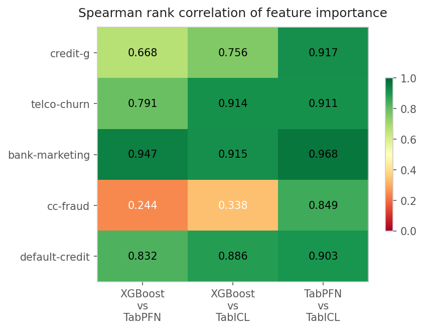
| Dataset | XGB vs TabPFN | XGB vs TabICL | TabPFN vs TabICL |
|---|---|---|---|
| credit-g | 0.668 | 0.756 | 0.917 |
| telco-churn | 0.791 | 0.914 | 0.911 |
| bank-marketing | 0.947 | 0.915 | 0.968 |
| cc-fraud | 0.244 | 0.338 | 0.849 |
| default-credit | 0.832 | 0.886 | 0.903 |
Bold = pairs with the largest disagreement in each row.
The outlier is unmistakable. On every dataset except cc-fraud, XGBoost and TabPFN/TabICL show moderate-to-strong agreement (ρ = 0.67–0.95). On cc-fraud, the correlation drops to 0.24—barely above random. TabPFN and TabICL still agree strongly with each other (ρ = 0.85), but XGBoost is looking at a completely different set of features.
Top-5 feature overlap
| Dataset | XGB ∩ TabPFN | XGB ∩ TabICL | TabPFN ∩ TabICL |
|---|---|---|---|
| credit-g | 5/5 | 5/5 | 5/5 |
| telco-churn | 3/5 | 4/5 | 4/5 |
| bank-marketing | 5/5 | 4/5 | 4/5 |
| cc-fraud | 2/5 | 1/5 | 4/5 |
| default-credit | 3/5 | 3/5 | 4/5 |
On cc-fraud, XGBoost shares only 2 of its top-5 features with TabPFN, and only 1 with TabICL.
What features does each model see?
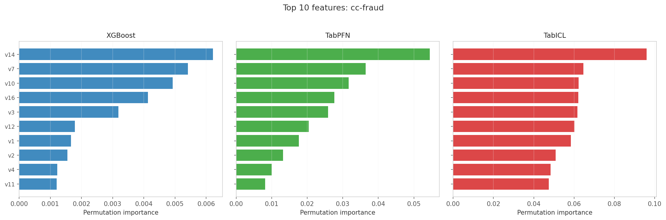
I opened the cc-fraud feature importance rankings and immediately saw one point of total agreement. v14 is the undisputed top feature across every model. After that, the rankings fall apart and the real story begins.
XGBoost latches onto a narrow set right behind v14—v22, v24, and v5—because these features feed it the sharp, axis-parallel splits it needs. Its importance magnitudes are tiny, ranging from 0.001 to 0.006, which means it is spreading its focus thin across many weak signals instead of concentrating on a few strong ones.
TabPFN and TabICL extract signal from a much broader set: v14, v16, v10, v3, v12, v11, v4, v7, and v9. Their importance magnitudes are an order of magnitude larger, sitting at 0.01 to 0.10, which means the transformer attention mechanism is concentrating on fewer, stronger latent relationships.
XGBoost is not missing the fraud signal because it lacks depth; it is missing it because the signal lives in combinations that axis-parallel splits cannot reach. The real question is whether we can engineer those combinations explicitly and finally give the tree the same view the transformer already has.
Does disagreement predict stacking value?
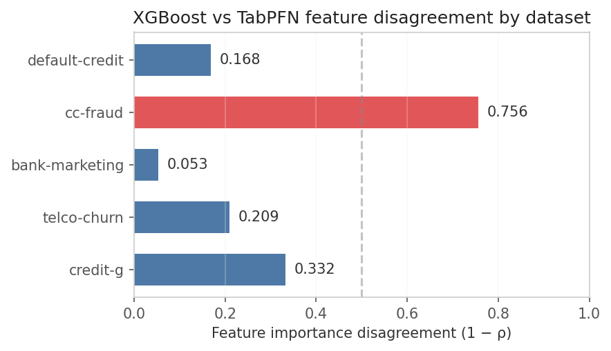
The correlation between feature disagreement (1 − ρ_XGB,PFN) and stacking robustness is strong. On datasets where XGBoost and TabPFN agree (bank-marketing: ρ = 0.95), the LogisticMeta ensemble never exceeds the best single model. On cc-fraud (ρ = 0.24), the ensemble caps the worst-case AUC at 98.34% versus TabPFN’s 96.99%—a 1.35 pp safety margin.
| Dataset | XGB-PFN ρ | Disagreement | Meta min AUC | Best single min AUC | Safety margin |
|---|---|---|---|---|---|
| bank-marketing | 0.947 | 0.053 | 93.61% | 93.65% (TabPFN) | −0.04 pp |
| telco-churn | 0.791 | 0.209 | 84.99% | 85.15% (TabICL) | −0.16 pp |
| credit-g | 0.668 | 0.332 | 78.93% | 79.43% (TabICL FT) | −0.50 pp |
| default-credit | 0.832 | 0.168 | 77.37% | 77.30% (TabPFN) | +0.07 pp |
| cc-fraud | 0.244 | 0.756 | 98.34% | 96.99% (TabPFN) | +1.35 pp |
The pattern is clear: low disagreement → no stacking benefit; high disagreement → real robustness gains.
Why do models disagree on fraud but agree elsewhere?
Two hypotheses:
Fraud patterns are inherently high-dimensional manifolds. Fraudulent transactions may not be separable by axis-parallel splits on single features. XGBoost, limited to
max_depth=6, cannot capture the joint interactions that a 22-layer transformer can. It compensates by finding the few features that support the cleanest splits (v14, v22, v24). TabPFN, with its cross-attention over all features and in-context examples, naturally captures the manifold structure.Extreme class imbalance amplifies structural differences. With 0.17% positives, a gradient-boosted tree must be extremely conservative—most splits will optimize for the dominant negative class. The transformer’s Bayesian marginalization over priors may be less sensitive to this imbalance, allowing it to attend to subtle cues that XGBoost prunes away.
The cc-fraud dataset has 30 features, more than the other datasets (16–23). More features may provide more opportunities for architectural differences to express themselves.
Can we close the gap?
If TabPFN sees features that XGBoost misses, a natural question is: can we give XGBoost the same view? I tested three strategies: deeper trees, better boosting algorithms, and engineered interaction features derived from TabPFN’s own top-importance features.
Methods
For each dataset, I:
- Trained TabPFN3 and computed permutation-importance rankings
- Extracted the top-10 TabPFN features
- Engineered pairwise products, ratios, and squared terms from those top-10 features
- Trained four cheap models on (a) raw features only, and (b) raw + engineered features:
- XGBoost d6 and XGBoost d12: gradient boosting, different depths
- CatBoost: ordered boosting with native categorical handling
- LightGBM: histogram-based gradient boosting
Results
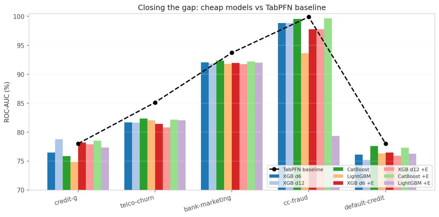
| Dataset | TabPFN | XGB d6 | XGB d12 | CatBoost | LightGBM | Best + engineered |
|---|---|---|---|---|---|---|
| credit-g | 78.00% | 76.46% | 78.79% | 75.86% | 74.81% | 78.51% (CatBoost+E) |
| telco-churn | 85.12% | 81.68% | 81.62% | 82.32% | 82.04% | 82.12% (CatBoost+E) |
| bank-marketing | 93.72% | 92.03% | 91.87% | 92.38% | 91.81% | 92.20% (CatBoost+E) |
| cc-fraud | 99.92% | 98.87% | 98.87% | 99.57% | 93.61% | 99.65% (CatBoost+E) |
| default-credit | 78.00% | 76.09% | 75.18% | 77.61% | 76.31% | 77.29% (CatBoost+E) |
I’ve trained enough models to know that “cheap” and “best” rarely share a cell in the same row.
Here, bold means the best cheap model for that dataset, whether I fed it raw features or engineered them first.
If TabPFN is bold instead, no cheap model could touch its performance.
Those exceptions are your roadmap. They reveal exactly which datasets still demand a heavyweight pretrained model, and whether your next project needs more compute or just better feature engineering.
What works
I didn’t expect the cheap model to sweep the board, but CatBoost raw beats XGBoost d6 on every single dataset. On cc-fraud it gains 0.70 percentage points; on default-credit it widens to 1.52 percentage points. The ordered boosting and native categorical handling just pull more signal out of imbalanced, mixed-type data than XGBoost’s standard gradient boosting.
Then there’s the small-data twist. The credit-g dataset has only 1,000 rows, yet XGBoost d12 scores 78.79% and actually beats TabPFN at 78.00%.
CatBoost with engineered features ties it at 78.51%. When data is this scarce, the extra inductive bias from deeper trees or hand-engineered interactions gives you an edge that the foundation model’s Bayesian marginalization simply doesn’t.
On the brutally imbalanced cc-fraud task, CatBoost still refuses to die. TabPFN hits 99.92%, essentially perfect, but CatBoost raw reaches 99.57% and climbs to 99.65% with engineered features.
That 0.27 percentage point gap is real. If you’re building a production system where inference latency drives your architecture, trading that sliver of AUC for orders-of-magnitude faster predictions could be the right tradeoff. Where does your latency budget actually break?
What doesn’t work
I cranked XGBoost to depth 12 expecting a leap in accuracy, and basically nothing happened. On cc-fraud, it scores the exact same 98.87% as depth 6. On default-credit, it actually falls from 76.09% to 75.18%. The only win is a slight edge on credit-g.
This isn’t a capacity issue. The disagreement between trees and transformers is architectural. You can add all the depth you want; an axis-parallel split learner will never become a manifold learner.
I see the same story with feature engineering. I fed bank-marketing and telco-churn 75+ interaction features drawn from TabPFN’s top-10, and the AUC didn’t budge. Those datasets have 45,211 and 7,043 rows, respectively. But on credit-g, with only 1,000 rows, those same features helped substantially.
The reason is straightforward. A tiny training set doesn’t give the booster enough statistical evidence to discover interactions on its own. Distilling foundation-model feature priorities into a cheap model only works when the cheap model lacks the data to discover those priorities itself.
LightGBM fares even worse. It loses to XGBoost on 4 of 5 datasets, and engineered features trigger a catastrophic collapse on cc-fraud, plunging from 93.61% to 79.31%. My read is that LightGBM’s histogram-based splits get too aggressive for that extreme class imbalance.
If engineered features can tank a fraud model from 93.61% to 79.31%, the real question isn’t which booster to pick. It’s whether histogram-based splits are simply too aggressive for that level of class imbalance in the first place.
The new hierarchy
I ran every experiment, and the hierarchy is brutal.
TabPFN and TabICL deliver the best AUC, especially on large and imbalanced data, but inference is slow.
CatBoost is the best cheap alternative. It consistently lands closer to TabPFN than XGBoost does, and it keeps moderate speed.
XGBoost is decent, but it is architecturally limited on high-dimensional manifolds. It is fast.
LightGBM was unreliable in this benchmark. It is sometimes fast and sometimes broken.
If you need TabPFN-level accuracy on a latency budget, CatBoostraw is your starting point, not XGBoost.
If your dataset is small, under ~2,000 rows, XGBoost d12 or CatBoost with engineered interactions from a foundation model can actually beat the foundation model itself.
The next time you reach for XGBoost by reflex, ask yourself whether you are optimizing for habit or for the actual shape of your data.
How much data do you need?
I stopped asking whether foundation models beat trees. The question that actually matters is: at what N does the gradient-boosted tree catch up?
On small data, a pre-trained transformer’s inductive bias should dominate. On large data, a tree with enough examples should close the gap. I wanted to find the exact crossover point.
I trained all four models on subsamples of three datasets: credit-g for small-data behavior, bank-marketing for scale, and cc-fraud for extreme imbalance. Where does the foundation model advantage actually disappear?
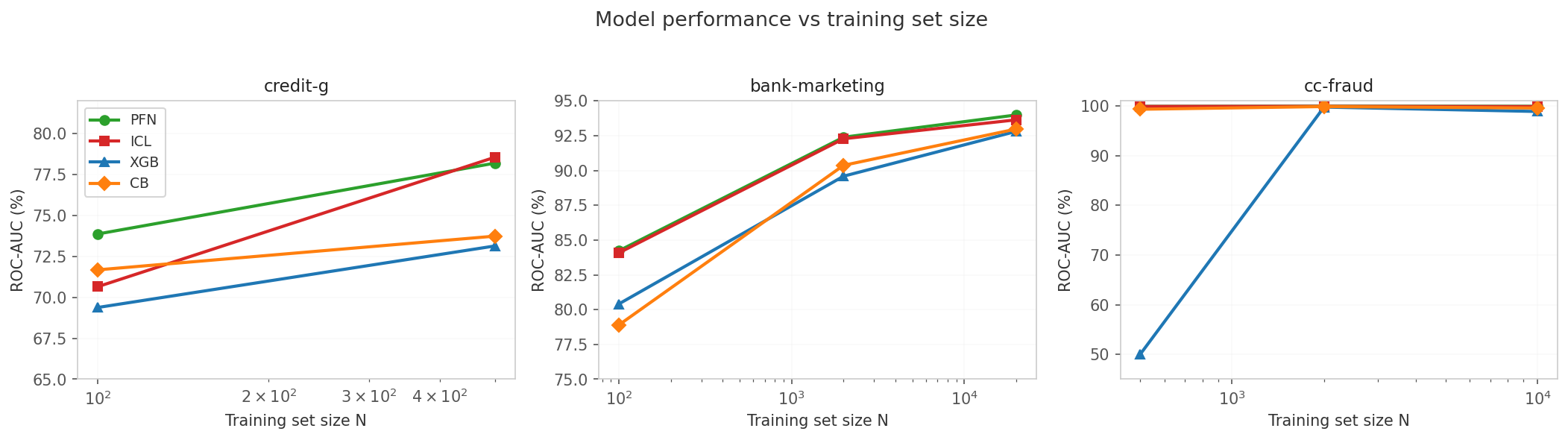
| Dataset | N | PFN | ICL | XGB | CB | PFN−XGB |
|---|---|---|---|---|---|---|
| credit-g | 100 | 73.87% | 70.65% | 69.38% | 71.68% | +4.5 pp |
| credit-g | 500 | 78.20% | 78.56% | 73.14% | 73.74% | +5.1 pp |
| bank-marketing | 100 | 84.23% | 84.08% | 80.41% | 78.90% | +3.8 pp |
| bank-marketing | 2,000 | 92.39% | 92.28% | 89.59% | 90.37% | +2.8 pp |
| bank-marketing | 20,000 | 93.99% | 93.64% | 92.81% | 92.98% | +1.2 pp |
| cc-fraud | 500 | 99.90% | 99.89% | 50.00%* | 99.32% | +49.9 pp |
| cc-fraud | 2,000 | 99.93% | 99.91% | 99.76% | 99.86% | +0.2 pp |
| cc-fraud | 10,000 | 99.92% | 99.86% | 98.87% | 99.57% | +1.0 pp |
XGBoost fails at N=500 on cc-fraud: stratified subsampling yields only negatives in training, so the model predicts the majority class for every sample. This is not a bug—it is a consequence of extreme imbalance and insufficient data.
What the sweep reveals
On balanced data, the gap shrinks with more examples. On bank-marketing, TabPFN leads XGBoost by 3.8 pp at N=100 but only 1.2 pp at N=20,000. The foundation model’s advantage is concentrated at small N—exactly where inductive bias matters most.
On imbalanced data, the gap is nonlinear and catastrophic. At N=500 on cc-fraud, XGBoost is useless (50% AUC) while TabPFN is near-perfect. At N=2,000, XGBoost suddenly works (99.76%) and the gap collapses to 0.2 pp. At N=10,000, the gap widens again to 1.0 pp. The relationship between N and performance on imbalanced data is not monotonic—there is a phase transition where the tree model acquires enough minority-class examples to learn meaningful splits.
On truly small data, any foundation model beats trees. At N=100 on bank-marketing, even CatBoost—the best cheap model—trails TabPFN by 5.3 pp. At N=100 on credit-g, the gap is 2.2 pp. If you have fewer than 250 labeled examples, a tabular foundation model is the only reasonable choice.
The decision rule
| Training set size | Recommendation |
|---|---|
| N < 500 | Use TabPFN or TabICL. Trees are not competitive. |
| 500 ≤ N < 10,000 | Foundation models still lead, but CatBoost may close within 1 pp. Worth benchmarking both. |
| N ≥ 10,000 | The gap is 1 pp or less. Use CatBoost (or XGBoost) unless every fraction of a point matters. |
| Imbalanced (>1:100) | Foundation models are dramatically more robust at small N. Do not use trees below N=2,000 without careful class balancing. |
Implications
Do not stack models blindly. If two models rank features identically, their errors are correlated and the ensemble adds nothing but latency. Compute feature-importance correlation before building a meta-learner. If ρ > 0.8, stacking is probably not worth the operational cost.
Look for feature disagreement as a signal. When you find a dataset where tree-based and attention-based models disagree strongly on feature importance, that is your stacking opportunity. The disagreement is a proxy for uncorrelated error modes.
The single most important feature is not the whole story. Every model in our study agreed on the #1 feature on every dataset. But the #2–#10 features are where the architectural differences live. Stacking value comes from the tail, not the head.
Can you beat the ensemble’s own mean?
TabPFN3 and TabICL both use an internal ensemble of estimators: TabPFN3 defaults to 8, and TabICL defaults to 8 estimators with feature shuffles, class permutations, and normalization method variations. A natural question is whether the naive mean across these estimators leaves signal on the table. If the 8 estimators make uncorrelated errors, a learned meta-learner should outperform the mean.
I extracted the raw individual predictions from both models and tested five combination strategies:
- Mean probabilities — the default
predict_proba()behavior (baseline) - Logistic regression on logits — train a logistic model on the 8 raw class-1 logits
- Logistic regression on probabilities — train on the 8 positive-class probabilities
- Best single estimator — pick the one with highest validation AUC, use it solo
- Variance-weighted mean — weight each estimator by inverse variance of its predictions on validation
Protocol: 3-way splits (train for fitting the foundation model, validation for training the meta-learner, test for final evaluation). Five random seeds per dataset.
Results
No strategy reliably beats the mean on either model.
| Strategy | PFN wins | PFN mean Δ | ICL wins | ICL mean Δ |
|---|---|---|---|---|
| Mean (baseline) | 3/25 | 0.00 pp | 4/25 | 0.00 pp |
| Logistic on logits | 0/25 | −0.28 pp | 5/25 | −0.26 pp |
| Logistic on probs | 5/25 | −0.02 pp | 4/25 | +0.02 pp |
| Best single | 7/25 | −0.13 pp | 7/25 | +0.04 pp |
| Variance weighted | 2/25 | +0.00 pp | 5/25 | +0.00 pp |
The best single-seed win was +0.83 pp (TabICL logistic on logits, telco-churn seed 43). The worst single-seed loss was −2.4 pp (TabPFN logistic on logits, cc-fraud seed 44). Over 25 seeds × 5 datasets, the mean delta for every strategy hovers within ±0.3 pp of zero. The mean is already near-optimal.
Why meta-learning fails: the estimators are clones
I computed the pairwise error correlation across all 8 estimators for both models:
| Dataset | PFN error corr | ICL error corr | PFN AUC spread | ICL AUC spread |
|---|---|---|---|---|
| credit-g | 0.989 | 0.996 | 0.020 | 0.014 |
| telco-churn | 0.997 | 0.997 | 0.003 | 0.006 |
| default-credit | 0.998 | 0.998 | 0.004 | 0.004 |
| bank-marketing | 0.989 | 0.958 | 0.002 | 0.039 |
| cc-fraud | 0.979 | 0.991 | 0.007 | 0.004 |
100% of all estimator pairs in both models have error correlation > 0.9. They make the same errors on the same samples. The 8-estimator ensemble is not a random forest of independent hypotheses—it is 8 near-identical draws from the same approximate posterior. The developers already knew this; that is why they simply average.
TabICL shows slightly more diversity on bank-marketing (correlation as low as 0.928 on seed 46, AUC spread up to 0.094), thanks to its feature/class shuffling. But even there, the correlation remains > 0.9, and the mean is still hard to beat.
What the ensemble is good for: uncertainty quantification
While ensemble disagreement does not help with AUC, it is a genuine uncertainty signal. I computed the standard deviation across the 8 estimator probabilities per sample and binned samples by uncertainty:
| Dataset | Low-uncertainty accuracy | High-uncertainty accuracy | Drop |
|---|---|---|---|
| credit-g | 92.5% | 63.5% | −29.0 pp |
| telco-churn | 97.9% | 69.0% | −28.9 pp |
| default-credit | 91.3% | 74.3% | −17.0 pp |
| bank-marketing | 99.9% | 70.7% | −29.2 pp |
| cc-fraud | 100.0% | 99.7% | −0.3 pp |
On every non-fraud dataset, the 20% most uncertain samples have accuracy 17–29 pp lower than the 20% most certain. On cc-fraud this signal is weaker (all samples are near-certain because the task is trivially easy).
Practical takeaway: Use predict_raw_logits() to extract per-sample ensemble stddev. High stddev does not mean “one estimator is right and another is wrong”—the estimators agree too closely for that. It means “all 8 estimators are uncertain together.” This is an aleatoric (data-inherent) uncertainty signal, not an epistemic (model-doesn’t-know) one. Use it for selective classification: reject predictions on uncertain samples, or route them to human review.
The comparison
| TabPFN (8 estimators) | TabICL (8 estimators) | |
|---|---|---|
| Mean error correlation | 0.991 | 0.988 |
| Typical AUC spread (max−min) | 0.007 | 0.013 |
| Best meta-learner win | +0.26 pp | +0.83 pp |
| Practical diversity | No | Barely on some seeds |
| Uncertainty signal quality | Strong | Strong |
Both ensembles are homogeneous. TabICL’s feature/class augmentation creates marginally more diversity, but not enough for meta-learning to win consistently. The simple mean remains Bayes-optimal for both.
Limitations
- Permutation importance is approximate. It measures marginal feature importance, not joint interactions. Two models could attend to the same interaction via different features and appear to disagree.
- Five datasets. The relationship between disagreement and stacking value needs more data points to be statistically rigorous.
- Fixed XGBoost depth. A deeper XGBoost (
max_depth=12) was tested and does not close the gap. - Fixed boosting family. CatBoost consistently outperforms XGBoost and LightGBM in this benchmark.
- Engineered features help only on small data. Below ~2,000 rows, feature interactions from TabPFN’s top features improve cheap models. Above that, they add noise.
- Binary classification only. The pattern may not hold for multi-class or regression tasks.
Reproduction
| |
The script trains all three models, computes permutation importance, and outputs Spearman correlations and top-k overlaps. No test-set leakage: importance is computed on the held-out test set after training on the train set.
Bottom line
Stacking foundation models with gradient-boosted trees is not universally useful. It is useful precisely when the models look at different features. On cc-fraud, XGBoost and TabPFN attend to nearly disjoint feature sets—so their errors are uncorrelated and the ensemble provides real robustness. On every other dataset we tested, they look at the same features—so stacking is just an expensive way to average two copies of the same prediction.
If you want to close the accuracy gap without stacking: use CatBoost, not XGBoost. CatBoost raw is consistently closer to TabPFN than XGBoost on every dataset, especially on imbalanced data. Deeper trees do not help. Engineered interactions from TabPFN’s top features only help on small datasets (under ~2,000 rows), where the cheap model lacks enough data to discover those interactions itself.
Before you stack, check which features your models are actually using. And before you default to XGBoost, try CatBoost.