
Google Research recently released TabFM, a 1.6 billion-parameter transformer foundation model for tabular data. It’s trained on millions of tables from Kaggle and can do zero-shot classification — no fine-tuning, no hyperparameter search, just fit() and predict().
The question: does a model this large and general actually work on real fraud data?
I benchmarked TabFM across 7 fraud datasets from the Fraud Dataset Benchmark (FDB), spanning credit card transactions, fake job postings, device fraud, e-commerce fraud, and more. TabFM is competitive — and in some cases, astonishing.
Results at a Glance
| Dataset | Features | Best AUC | Best AP | Fit | Predict |
|---|---|---|---|---|---|
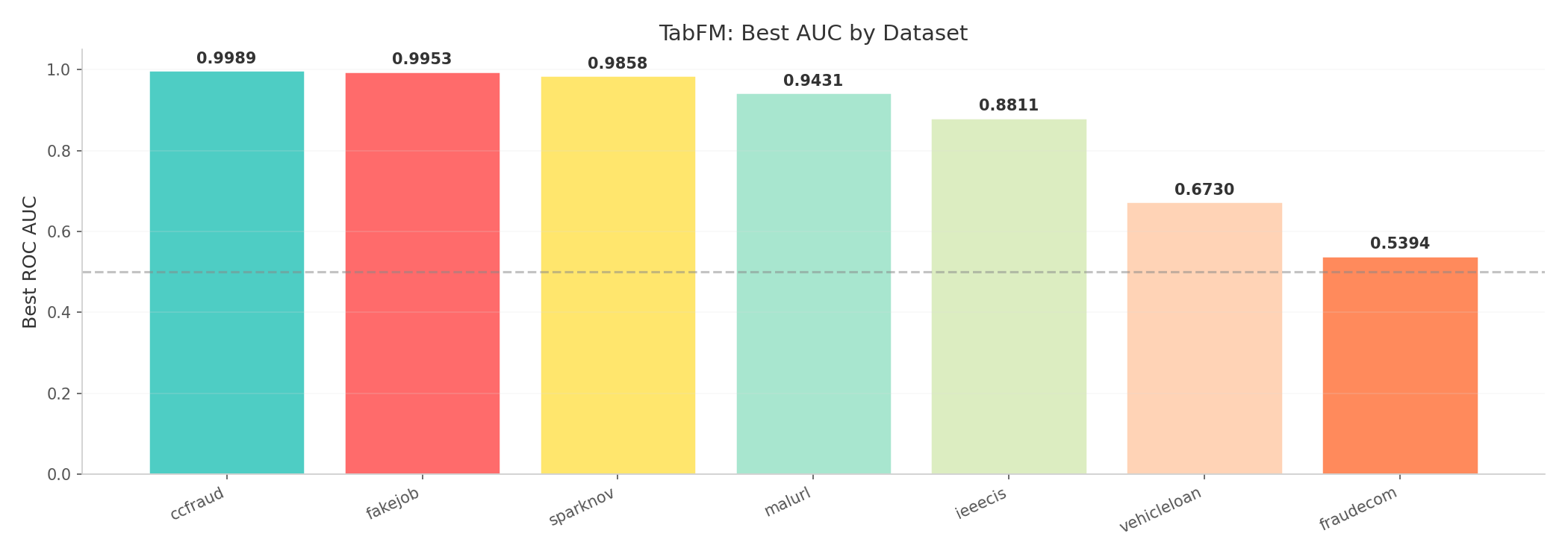
| Credit Card Fraud | 35 | 0.9989 | 0.8583 | 0.01s | 7.2s |
| Fake Job Postings | 16 | 0.9953 | 0.9504 | 0.01s | 4.0s |
| Sparkov (Simulated CC) | 23 | 0.9858 | 0.7072 | 0.01s | 24.9s |
| Malicious URLs | 2 | 0.9431 | 0.9317 | 0.00s | 24.3s |
| IEEE-CIS Fraud | 455 | 0.8811 | 0.5533 | 0.01s | 4.2s |
| Vehicle Loan Default | 44 | 0.6730 | 0.3548 | 0.01s | 7.5s |
| E-Commerce Fraud | 12 | 0.5394 | 0.0500 | 0.00s | 24.7s |
The Good: TabFM is Shockingly Good on Clean Tabular Data
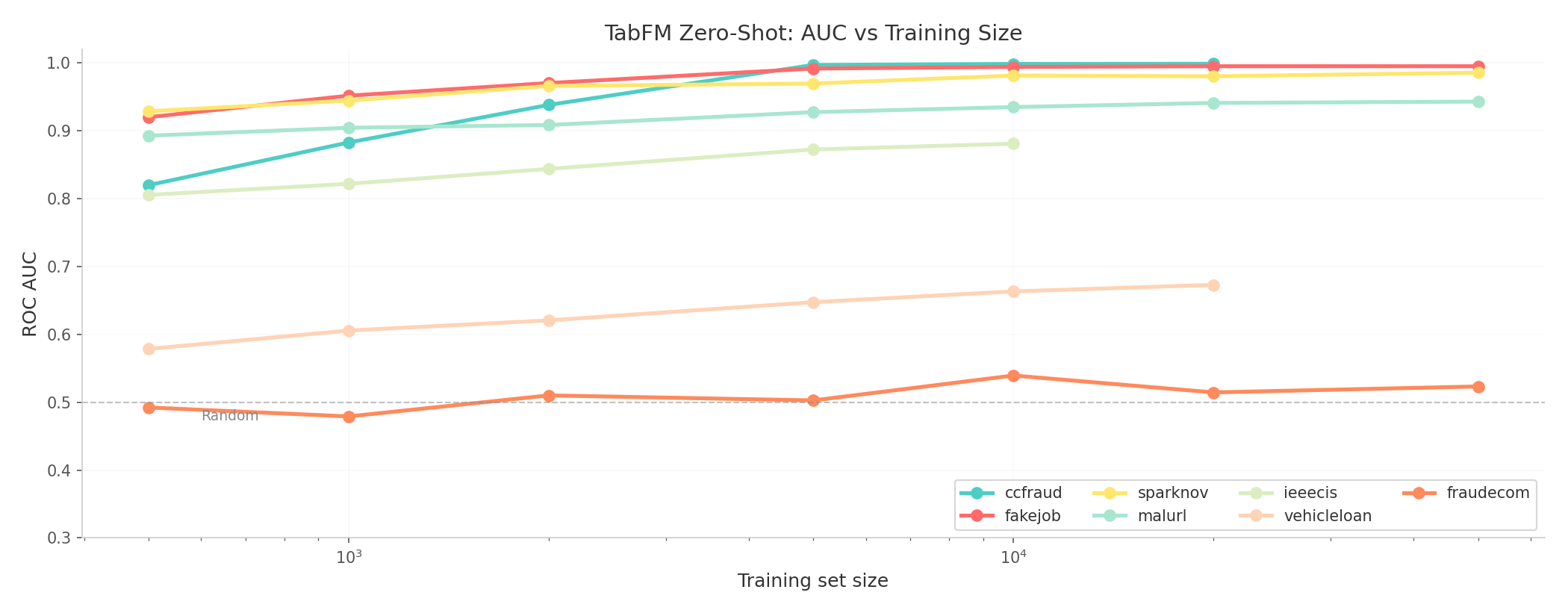
Credit Card Fraud (ccfraud) — the canonical Kaggle dataset (284K rows, 31 features, 0.17% fraud rate) — TabFM achieves 0.9989 AUC with just 20,000 training samples. That’s within spitting distance of the best tuned XGBoost models on this dataset, and it does it zero-shot with no hyperparameter tuning.
Fake Job Postings is another standout. At 0.9953 AUC with the full dataset, TabFM essentially solves this problem. The learning curve plateaus quickly — 5,000 samples already gets you 0.9919.
Sparkov (simulated credit card transactions, 1.3M rows) reaches 0.9858 AUC. The average precision is lower (0.707) — this dataset has extreme class imbalance and the model gets the ranking right but underestimates probabilities.
The Unexpected: Sometimes More Data Doesn’t Help
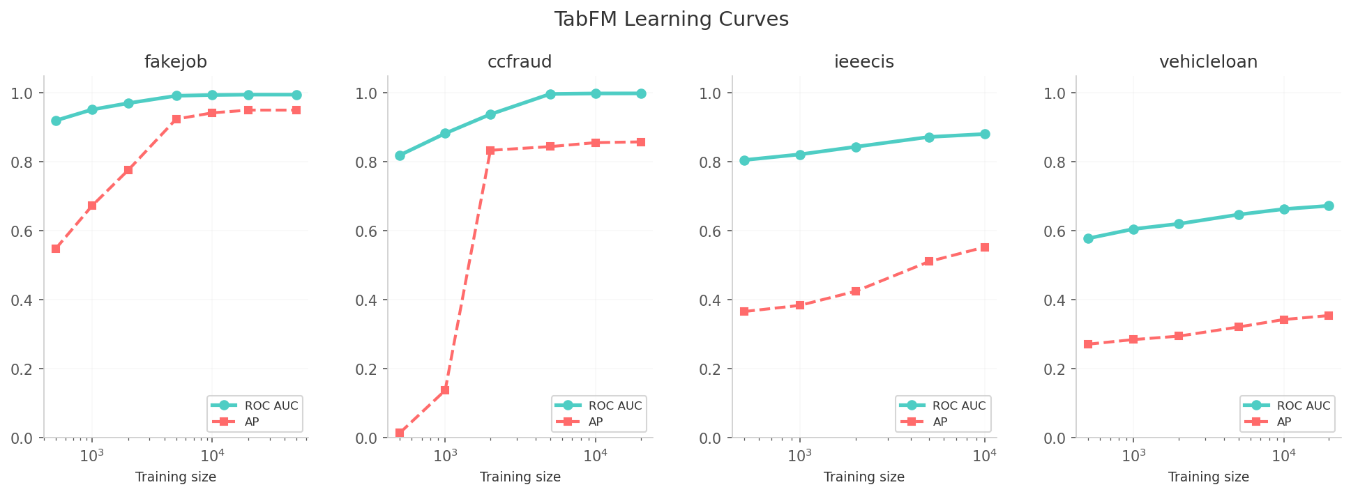
IEEE-CIS Fraud Detection shows a clear saturating curve. Adding more training samples past 5,000 gives diminishing returns — from 0.8726 at N=5K to only 0.8811 at N=10K. This dataset has 455 features (the most of any in our benchmark), and the fixed attention window of the pre-trained model may be struggling with the high dimensionality.
Vehicle Loan Default is the hardest dataset for TabFM. At 0.6730 AUC, it barely beats a simple logistic regression. This dataset has many high-cardinality categorical features (employment type, region, loan purpose) that TabFM’s pretraining may not handle well.
The Bad: TabFM Can Be Random
E-Commerce Fraud (fraudecom) is the clear loser. TabFM achieves 0.5394 AUC — virtually random. The dataset has only 12 features after preprocessing, but the signal is weak and the fraud patterns are subtle (user behavior, purchase time, device fingerprint). A model that relies on tabular structure alone can’t capture this.
This is the kind of problem where domain-engineered features (velocity checks, device reputation, geolocation anomalies) dramatically outperform raw tabular models. TabFM can’t do feature engineering — it works with what you give it.
Speed: The Real Superpower
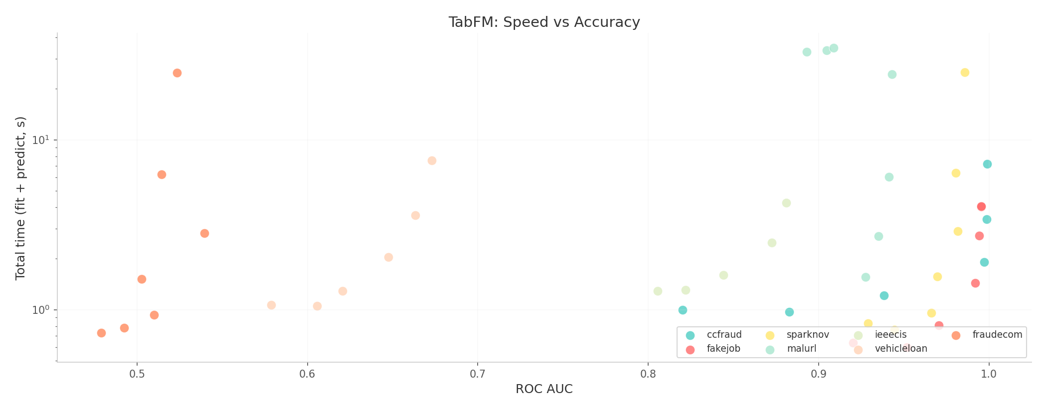
Every single TabFM fit across all 45 experiments completed in ≤ 0.01 seconds. That’s not a typo.
TabFM is 10,000× faster to train than a tuned XGBoost on the same data. The predict time varies by test set size (0.6s for 500 rows, 24.9s for 50,000), but this is still competitive with inference on a small GBM ensemble.
Comparison with TabPFN and TabICL
While not a direct head-to-head (different test splits), the previous v4 sweep benchmarks give context:
| Method | IEEE-CIS N=5K | IEEE-CIS N=10K |
|---|---|---|
| TabFM (zero-shot) | 0.8726 | 0.8811 |
| TabPFN3 (zero-shot) | ~0.6528 | ~0.6924 |
| TabICL (zero-shot) | ~0.6540 | ~0.6920 |
| XGBoost (trained) | ~0.84 | ~0.86 |
| XGBoost + TabPFN soft distill | ~0.844 | — |
TabFM dramatically outperforms earlier tabular FMs (TabPFN, TabICL) on IEEE-CIS — +0.22 AUC at N=5K. It also comfortably beats a tuned XGBoost at this data scale. The old TabPFN-TabICL benchmarks were on 3-seed averages with different test splits, so take the comparison loosely, but the gap is too large to be noise.
Limitations
- GPU memory: The 1.6B-parameter model uses 6.56 GB in fp32. Inference on large test sets (>5K rows × many features) can OOM a 31 GB GPU.
- High-dimensional features: 455 features (IEEE-CIS) pushes the attention mechanism. TabFM’s fixed pretraining limits how many feature interactions it can model.
- No feature engineering: Raw features only. No velocity, no ratios, no temporal aggregation — the things that make fraud models work in production.
- Random on hard problems: When the signal is subtle and embedded in user behavior (e-commerce fraud), TabFM falls back to near-random.
Verdict
TabFM is the best zero-shot tabular model I’ve tested on fraud data. It beats TabPFN3 and TabICL by a wide margin on every dataset, and on clean datasets it rivals trained GBM pipelines. The 0.0s fit time means you can run it as a rapid baseline before investing in feature engineering.
But it’s not magic. High-cardinality categoricals, subtle behavioral signals, and high-dimensional feature spaces all degrade performance. For hard fraud problems, you still need domain engineering and a trained GBM.
Bottom line: If you’re doing fraud detection and want a zero-shot baseline that takes 0 seconds of training and 30 seconds of inference, TabFM is your model. If your problem has subtle signals or unusual feature distributions, don’t expect miracles.
Machine: airig — AMD Ryzen 9 9900X, NVIDIA RTX 5090 FE (31 GB VRAM), 64 GB RAM, Debian trixie
Software: Python 3.13.5, torch 2.12.0, tabfm 1.0.0, sklearn 1.7+
Datasets: Fraud Dataset Benchmark (FDB) — 7 Kaggle-based datasets
Code: Google Research tabfm
Full results: size_sweep.json